Šajā apmācībā mēs apspriedīsim dažādus veidus, kā mēs varam izveidot matricu, izmantojot Python, kā arī apspriedīsim dažādas darbības, kuras var veikt ar matricu. mēs apskatīsim arī ārējo moduli Numpy, lai izveidotu matricu, un tās darbības Python.
Kas ir matrica?
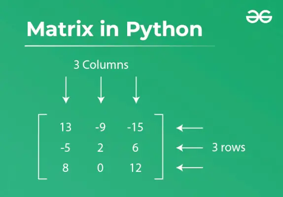
Matrica ir skaitļu kopums, kas sakārtots taisnstūra masīvā rindās un kolonnās. Inženierzinātņu, fizikas, statistikas un grafikas jomās matricas plaši izmanto, lai izteiktu attēlu rotācijas un cita veida transformācijas.
Matrica tiek apzīmēta kā m ar n matrica, ko apzīmē ar simbolu m x n ja ir m rindas un n kolonnas.
Vienkāršas matricas izveide, izmantojot Python
1. metode: matricas izveide ar sarakstu sarakstu
Šeit mēs izveidosim matricu, izmantojot sarakstu sarakstu.
Python3
virknē java
matrix>=> [[>1>,>2>,>3>,>4>],> >[>5>,>6>,>7>,>8>],> >[>9>,>10>,>11>,>12>]]> print>(>'Matrix ='>, matrix)> |
>
>
Izvade:
Matrix = [[1, 2, 3, 4], [5, 6, 7, 8], [9, 10, 11, 12]]>
2. metode: ņemiet Matrix ievadi no lietotāja Python
Šeit mēs no lietotāja paņemam vairākas rindas un kolonnas un izdrukājam Matrix.
Python3
Row>=> int>(>input>(>'Enter the number of rows:'>))> Column>=> int>(>input>(>'Enter the number of columns:'>))> # Initialize matrix> matrix>=> []> print>(>'Enter the entries row wise:'>)> # For user input> # A for loop for row entries> for> row>in> range>(Row):> >a>=> []> ># A for loop for column entries> >for> column>in> range>(Column):> >a.append(>int>(>input>()))> >matrix.append(a)> # For printing the matrix> for> row>in> range>(Row):> >for> column>in> range>(Column):> >print>(matrix[row][column], end>=>' '>)> >print>()> |
>
>
Izvade:
Enter the number of rows:2 Enter the number of columns:2 Enter the entries row wise: 5 6 7 8 5 6 7 8>
Laika sarežģītība: O(n*n)
Papildtelpa: O(n*n)
3. metode: izveidojiet matricu, izmantojot saraksta izpratni
Saraksta izpratne ir elegants veids, kā definēt un izveidot sarakstu Python, mēs izmantojam diapazona funkciju 4 rindu un 4 kolonnu drukāšanai.
Python3
matrix>=> [[column>for> column>in> range>(>4>)]>for> row>in> range>(>4>)]> print>(matrix)> |
>
>
Izvade:
[[0, 1, 2, 3], [0, 1, 2, 3], [0, 1, 2, 3], [0, 1, 2, 3]]>
Vērtības piešķiršana matricā
1. metode: piešķiriet vērtību atsevišķai Matrix šūnai
Šeit mēs aizvietojam un piešķiram vērtību atsevišķai šūnai (1 rinda un 1 kolonna = 11) matricā.
Python3
X>=> [[>1>,>2>,>3>], [>4>,>5>,>6>], [>7>,>8>,>9>]]> row>=> column>=> 1> X[row][column]>=> 11> print>(X)> |
>
>
Izvade:
[[1, 2, 3], [4, 11 , 6], [7, 8, 9]]>
2. metode: piešķiriet vērtību atsevišķai šūnai, izmantojot negatīvu indeksāciju programmā Matrix
Šeit mēs aizvietojam un piešķiram vērtību atsevišķai šūnai (-2 rindas un -1 kolonna = 21) matricā.
Python3
masīvu saraksts
row>=> ->2> column>=> ->1> X[row][column]>=> 21> print>(X)> |
>
>
Izvade:
[[1, 2, 3], [4, 5, 21 ], [7, 8, 9]]>
Piekļuve vērtībai matricā
1. metode: piekļuve matricas vērtībām
Šeit mēs piekļūstam Matricas elementiem, nododot tās rindai un kolonnai.
Python3
print>(>'Matrix at 1 row and 3 column='>, X[>0>][>2>])> print>(>'Matrix at 3 row and 3 column='>, X[>2>][>2>])> |
>
>
Izvade:
Matrix at 1 row and 3 column= 3 Matrix at 3 row and 3 column= 9>
2. metode. Piekļuve matricas vērtībām, izmantojot negatīvu indeksāciju
Šeit mēs piekļūstam Matricas elementiem, nododot tās rindai un kolonnai negatīvai indeksācijai.
Python3
import> numpy as np> X>=> [[>1>,>2>,>3>], [>4>,>5>,>6>], [>7>,>8>,>9>]]> print>(X[>->1>][>->2>])> |
>
>
Izvade:
8>
Matemātiskās operācijas ar matricu Python
1. piemērs: vērtību pievienošana matricai ar for cilpu programmā python
Šeit mēs pievienojam divas matricas, izmantojot Python for-cilpu.
Python3
# Program to add two matrices using nested loop> X>=> [[>1>,>2>,>3>],[>4>,>5>,>6>], [>7>,>8>,>9>]]> Y>=> [[>9>,>8>,>7>], [>6>,>5>,>4>], [>3>,>2>,>1>]]> result>=> [[>0>,>0>,>0>], [>0>,>0>,>0>], [>0>,>0>,>0>]]> # iterate through rows> for> row>in> range>(>len>(X)):> ># iterate through columns> >for> column>in> range>(>len>(X[>0>])):> >result[row][column]>=> X[row][column]>+> Y[row][column]> for> r>in> result:> >print>(r)> |
>
>
Izvade:
[10, 10, 10] [10, 10, 10] [10, 10, 10]>
Laika sarežģītība: O(n*n)
Papildtelpa: O(n*n)
2. piemērs. Vērtību pievienošana un atņemšana matricai ar saraksta izpratni
Pamata saskaitīšanas un atņemšanas veikšana, izmantojot saraksta izpratni.
Python3
Add_result>=> [[X[row][column]>+> Y[row][column]> >for> column>in> range>(>len>(X[>0>]))]> >for> row>in> range>(>len>(X))]> Sub_result>=> [[X[row][column]>-> Y[row][column]> >for> column>in> range>(>len>(X[>0>]))]> >for> row>in> range>(>len>(X))]> print>(>'Matrix Addition'>)> for> r>in> Add_result:> >print>(r)> print>(>'
Matrix Subtraction'>)> for> r>in> Sub_result:> >print>(r)> |
>
>
Izvade:
Matrix Addition [10, 10, 10] [10, 10, 10] [10, 10, 10] Matrix Subtraction [-8, -6, -4] [-2, 0, 2] [4, 6, 8]>
Laika sarežģītība: O(n*n)
Papildtelpa: O(n*n)
3. piemērs: Python programma divu matricu reizināšanai un dalīšanai
Pamata reizināšanas un dalīšanas veikšana, izmantojot Python cilpu.
Python3
rmatrix>=> [[>0>,>0>,>0>], [>0>,>0>,>0>], [>0>,>0>,>0>]]> for> row>in> range>(>len>(X)):> >for> column>in> range>(>len>(X[>0>])):> >rmatrix[row][column]>=> X[row][column]>*> Y[row][column]> > print>(>'Matrix Multiplication'>,)> for> r>in> rmatrix:> >print>(r)> > for> i>in> range>(>len>(X)):> >for> j>in> range>(>len>(X[>0>])):> >rmatrix[row][column]>=> X[row][column]>/>/> Y[row][column]> print>(>'
Matrix Division'>,)> for> r>in> rmatrix:> >print>(r)> |
>
>
Izvade:
Matrix Multiplication [9, 16, 21] [24, 25, 24] [21, 16, 9] Matrix Division [0, 0, 0] [0, 1, 1] [2, 4, 9]>
Laika sarežģītība: O(n*n)
Papildtelpa: O(n*n)
Transponēt matricā
Piemērs: Python programma matricas transponēšanai, izmantojot cilpu
Matricas transponēšanu iegūst, mainot rindas uz kolonnām un kolonnas uz rindām. Citiem vārdiem sakot, A[][] transponēšana tiek iegūta, mainot A[i][j] uz A[j][i].
Python3
X>=> [[>9>,>8>,>7>], [>6>,>5>,>4>], [>3>,>2>,>1>]]> result>=> [[>0>,>0>,>0>], [>0>,>0>,>0>], [>0>,>0>,>0>]]> # iterate through rows> for> row>in> range>(>len>(X)):> ># iterate through columns> >for> column>in> range>(>len>(X[>0>])):> >result[column][row]>=> X[row][column]> for> r>in> result:> >print>(r)> > # # Python Program to Transpose a Matrix using the list comprehension> # rez = [[X[column][row] for column in range(len(X))]> # for row in range(len(X[0]))]> # for row in rez:> # print(row)> |
>
>
Izvade:
java konstantes
[9, 6, 3] [8, 5, 2] [7, 4, 1]>
Laika sarežģītība: O(n*n)
Papildtelpa: O(n*n)
Matrica, izmantojot Numpy
Izveidojiet matricu, izmantojot Numpy
Šeit mēs izveidojam Numpy masīvu, izmantojot numpy.random un a izlases modulis .
Python3
import> numpy as np> > # 1st argument -->skaitļi no 0 līdz 9,> # 2nd argument, row = 3, col = 3> array>=> np.random.randint(>10>, size>=>(>3>,>3>))> print>(array)> |
>
>
Izvade:
[[2 7 5] [8 5 1] [8 4 6]]>
Matricas matemātiskās darbības Python, izmantojot Numpy
Šeit mēs aplūkojam dažādas matemātiskās darbības, piemēram, saskaitīšanu, atņemšanu, reizināšanu un dalīšanu, izmantojot Numpy.
Python3
# initializing matrices> x>=> numpy.array([[>1>,>2>], [>4>,>5>]])> y>=> numpy.array([[>7>,>8>], [>9>,>10>]])> # using add() to add matrices> print> (>'The element wise addition of matrix is : '>)> print> (numpy.add(x,y))> # using subtract() to subtract matrices> print> (>'The element wise subtraction of matrix is : '>)> print> (numpy.subtract(x,y))> print> (>'The element wise multiplication of matrix is : '>)> print> (numpy.multiply(x,y))> # using divide() to divide matrices> print> (>'The element wise division of matrix is : '>)> print> (numpy.divide(x,y))> |
int dubultot
>
>
Izvade:
The element wise addition of matrix is : [[ 8 10] [13 15]] The element wise subtraction of matrix is : [[-6 -6] [-5 -5]] The element wise multiplication of matrix is : [[ 7 16] [36 50]] The element wise division of matrix is : [[0.14285714 0.25 ] [0.44444444 0.5 ]]>
Punkts un krustojums ar Matrix
Šeit mēs atradīsim matricu un vektoru iekšējo, ārējo un šķērsproduktu, izmantojot NumPy programmā Python.
Python3
X>=> [[>1>,>2>,>3>],[>4>,>5>,>6>],[>7>,>8>,>9>]]> Y>=> [[>9>,>8>,>7>], [>6>,>5>,>4>],[>3>,>2>,>1>]]> dotproduct>=> np.dot(X, Y)> print>(>'Dot product of two array is:'>, dotproduct)> dotproduct>=> np.cross(X, Y)> print>(>'Cross product of two array is:'>, dotproduct)> |
>
>
Izvade:
Dot product of two array is: [[ 30 24 18] [ 84 69 54] [138 114 90]] Cross product of two array is: [[-10 20 -10] [-10 20 -10] [-10 20 -10]]>
Matricas transponēšana Python, izmantojot Numpy
Lai veiktu transponēšanas operāciju matricā, mēs varam izmantot numpy.transpose() metodi.
Python3
matrix>=> [[>1>,>2>,>3>], [>4>,>5>,>6>]]> print>(>'
'>, numpy.transpose(matrix))> |
>
>
Izvade:
[[1 4][2 5][3 6]]>
Izveidojiet an tukša matrica ar NumPy programmā Python
Tukša masīva inicializācija, izmantojot np.zeros() .
Python3
a>=> np.zeros([>2>,>2>], dtype>=>int>)> print>(>'
Matrix of 2x2:
'>, a)> c>=> np.zeros([>3>,>3>])> print>(>'
Matrix of 3x3:
'>, c)> |
>
>
Izvade:
Matrix of 2x2: [[0 0] [0 0]] Matrix of 3x3: [[0. 0. 0.] [0. 0. 0.] [0. 0. 0.]]>
Sagriešana Matrix, izmantojot Numpy
Sagriešana ir process, kurā no matricas tiek atlasītas noteiktas rindas un kolonnas un pēc tam izveidota jauna matrica, noņemot visus neatlasītos elementus. Pirmajā piemērā mēs drukājam visu matricu, otrajā mēs nododam 2 kā sākotnējo indeksu, 3 kā pēdējo indeksu un indeksa lēcienu kā 1. Tas pats tiek izmantots nākamajā izdrukā, mēs tikko mainījām indeksu. pāriet uz 2.
Python3
X>=> np.array([[>6>,>8>,>10>],> >[>9>,>->12>,>15>],> >[>12>,>16>,>20>],> >[>15>,>->20>,>25>]])> # Example of slicing> # Syntax: Lst[ Initial: End: IndexJump ]> print>(X[:])> print>(>'
Slicing Third Row-Second Column: '>, X[>2>:>3>,>1>])> print>(>'
Slicing Third Row-Third Column: '>, X[>2>:>3>,>2>])> |
>
>
Izvade:
[[ 6 8 10] [ 9 -12 15] [ 12 16 20] [ 15 -20 25]] Slicing Third Row-Second Column: [16] Slicing Third Row-Third Column: [20]>
Dzēsiet rindas un kolonnas, izmantojot Numpy
Šeit mēs mēģinām dzēst rindas, izmantojot funkciju np.delete() . Kodā mēs vispirms mēģinājām izdzēst 0thrindu, tad mēģinājām dzēst 2ndrinda un pēc tam 3rdrinda.
Python3
# create an array with integers> # with 3 rows and 4 columns> a>=> np.array([[>6>,>8>,>10>],> >[>9>,>->12>,>15>],> >[>12>,>16>,>20>],> >[>15>,>->20>,>25>]])> # delete 0 th row> data>=> np.delete(a,>0>,>0>)> print>(>'data after 0 th row deleted: '>, data)> # delete 1 st row> data>=> np.delete(a,>1>,>0>)> print>(>'
data after 1 st row deleted: '>, data)> # delete 2 nd row> data>=> np.delete(a,>2>,>0>)> print>(>'
data after 2 nd row deleted: '>, data)> |
kā java ievadīt virkni uz int
>
>
Izvade:
data after 0 th row deleted: [[ 9 -12 15] [ 12 16 20] [ 15 -20 25]] data after 1 st row deleted: [[ 6 8 10] [ 12 16 20] [ 15 -20 25]] data after 2 nd row deleted: [[ 6 8 10] [ 9 -12 15] [ 15 -20 25]]>
Pievienojiet rindu/kolonnas masīvam Numpy
Mēs pievienojām vēl vienu kolonnu pie 4thpozīcija, izmantojot np.hstack .
Python3
ini_array>=> np.array([[>6>,>8>,>10>],> >[>9>,>->12>,>15>],> >[>15>,>->20>,>25>]])> # Array to be added as column> column_to_be_added>=> np.array([>1>,>2>,>3>])> # Adding column to numpy array> result>=> np.hstack((ini_array, np.atleast_2d(column_to_be_added).T))> # printing result> print>(>'
resultant array
'>,>str>(result))> |
>
>
Izvade:
resultant array [[ 6 8 10 1] [ 9 -12 15 2] [ 15 -20 25 3]]>